
Using the "Base Plate" component, you can design base plate connections with cast-in anchors. In addition to plates and welds, the design analyzes the anchorage and the steel-concrete interaction.
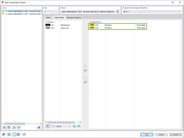
The combination wizard provides you with the option to consider more than one initial state. RFEM and RSTAB allow you to specify different initial states (prestress, form-finding, strain, and so on) for the target combinations in the combinatorics.
You can thus, for example, generate load states on the basis of a form-finding analysis with varying imperfections.
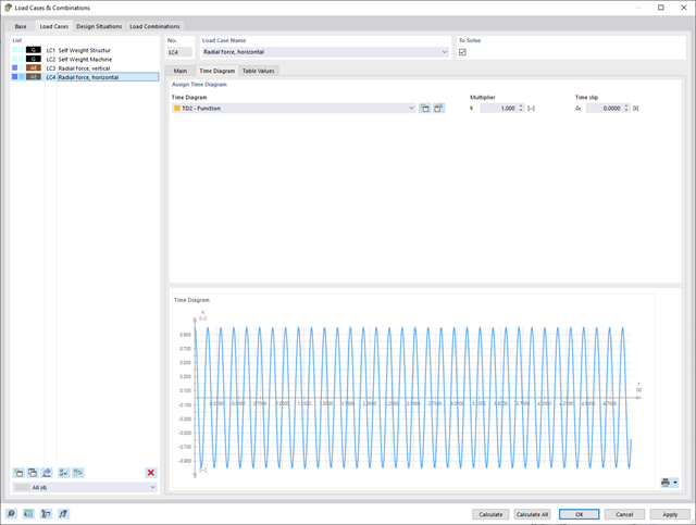
It is necessary to enter the required force-time diagrams. They can be combined in load cases or load combinations of the type Time History Analysis | Time Diagrams with the loading in order to define where and in which direction the force-time diagrams act.
The second option is to enter acceleration-time diagrams, which can be used in the load cases of the Time History Analysis | Accelerogram type.
All calculation parameters are specified in the time history analysis settings. These include, for example, the type of analysis method and the maximum calculation time.
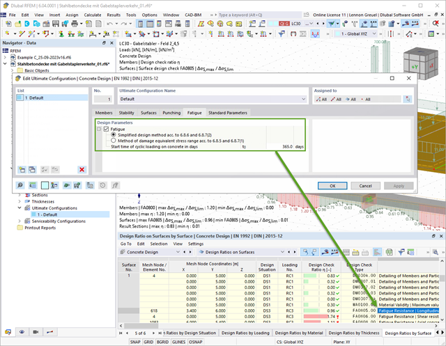
With the Concrete Design add-on, you can perform the fatigue design of members and surfaces according to EN 1992‑1‑1, Chapter 6.8.
For the fatigue design, you can optionally select two methods or design levels in the design configurations:
- Design Level 1: Simplified design according to 6.8.6 and 6.8.7(2): The simplified design is performed for frequent action combinations according to EN 1992‑1‑1, Chapter 6.8.6 (2), and EN 1990, Eq. (6.15b) with the traffic loads relevant in the serviceability state. A maximum stress range according to 6.8.6 is designed for the reinforcing steel. The concrete compressive stress is determined by means of the upper and lower allowable stress according to 6.8.7(2).
- Design Level 2: Design of damage equivalent stress acc. to 6.8.5 and 6.8.7(1) (simplified fatigue design): The design using damage equivalent stress ranges is performed for the fatigue combination according to EN 1992‑1‑1, Chapter 6.8.3, Eq. (6.69) with the specifically defined cyclic action Qfat.

The Ponding load type allows you to simulate rain actions on multi-curved surfaces, taking into account the displacements according to the large deformation analysis.
This numerical rainfall process examines the assigned surface geometry and determines which rainfall portions drain away and which rainfall portions accumulate in puddles (water pockets) on the surface. The puddle size then results in a corresponding vertical load for the structural analysis.
For example, you can use this feature in the analysis of approximately horizontal membrane roof geometries subjected to rain loading.
Go to Explanatory Video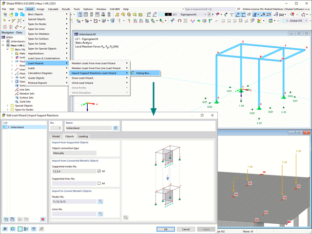
Use the "Import Support Reactions" Load Wizard in RFEM 6 and RSTAB 9 to easily transfer reaction forces from other models. The wizard allows you to connect all or several nodal and line loads of different models with each other in a few steps.
The load transfer from load cases and load combinations can be carried out automatically or manually. It's necessary that the models are saved in the same Dlubal Center project.
The "Import Support Reactions" load wizard supports the concept of positional statics and allows you to digitally connect the individual positions.
Go to Explanatory Video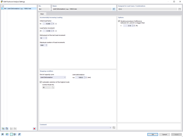
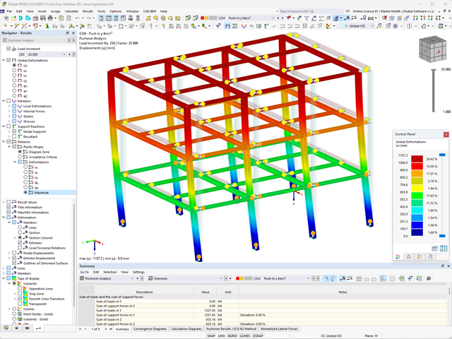
The pushover analysis is managed by a newly introduced analysis type in the load combinations. Here, you have access to the selection of the horizontal load distribution and direction, the selection of a constant load, the selection of the desired response spectrum for the determination of the target displacement, and the pushover analysis settings tailored to the pushover analysis.
In the pushover analysis settings, you can modify the increment of the increasing horizontal load and specify the stopping condition for the analysis. Furthermore, it is possible to easily adjust the precision for the iterative determination of the target displacement.
- Consideration of nonlinear component behavior using plastic standard hinges for steel (FEMA 356, EN 1998‑3) and nonlinear material behavior (masonry, steel - bilinear, user-defined working curves)
- Direct import of masses from load cases or combinations for the application of constant vertical loads
- User-defined specifications for the consideration of horizontal loads (standardized to a mode shape or uniformly distributed over the height of the masses)
- Determination of a pushover curve with selectable limit criterion of the calculation (a collapse or limit deformation)
- Transformation of the pushover curve into the capacity spectrum (ADRS format, single degree of freedom system)
- Bilinearization of the capacity spectrum according to EN 1998‑1:2010 + A1:2013
- Transformation of the applied response spectrum into the required spectrum (ADRS format)
- Determination of target displacement according to EC 8 (the N2 method according to Fajfar 2000)
- Graphical comparison of the capacity and required spectrum
- Graphical evaluation of the acceptance criteria of predefined plastic hinges
- Result display of the values used in the iterative calculation of the target displacement
- Access to all results of the structural analysis in the individual load levels
This function provides you with the option to adopt reaction forces from other models as nodal and line loads.
The option not only transfers the reaction load as an action, but digitally couples the support load of the original model with the load size of the target object. The subsequent changes in the original model are automatically adopted in the target model.
This technology supports the concept of positional statics and allows you to digitally connect the individual positions of the same Dlubal Center project.
Go to Explanatory Video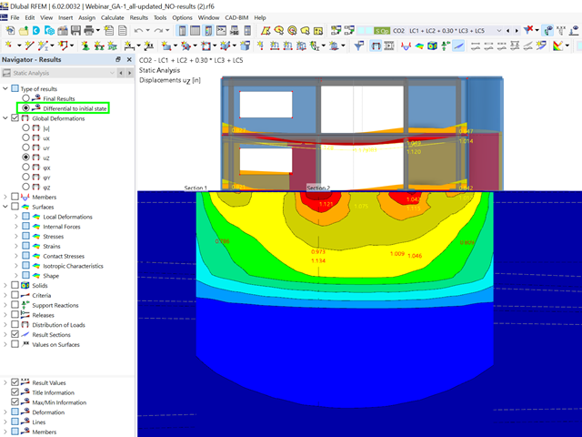
Did you already know? For load combinations, you can optionally display the difference results to the initial state. For example, you have the option for a geotechnical analysis to output the settlement as a difference to the initial state "soil self-weight".
.png?mw=640&hash=55038d2a1591f62179796666cb9b2fede0274e19)
A graphical and tabular output of the results for deformations, stresses, and strains helps you when determining the soil solids. To achieve this, use the special filter criteria for targeted selection of results.
The program doesn't leave you alone with the results. If you want to graphically evaluate the results in the soil solids, you can use the guide objects. For example, you can define clipping planes. This allows you to view the corresponding results in any plane of the soil solid.
And not just that. The utilization of result sections and clipping boxes facilitates the precise graphical analysis of the soil solid.
You already know that it is possible to model and analyze a soil and a structure in the entire model. As a result, you have explicitly taken into account the soil-structure interaction. By modifying a component, you achieve the immediate correct consideration in the analysis as well as in the results for the entire system of the soil and structure.

Are you ready for the evaluation? Use the calculation diagrams, which show the distribution of a specific result during the calculation.
You can freely define the layout of the vertical and horizontal axes of the calculation diagram. This allows you, for example, to consider the settlement distribution of a certain node, depending on the load.

Your data are always documented in a multilingual printout report. You can adjust the content at any time and save it as a template. You can also add graphics, texts, MathML formulas, and PDF documents to your report with just a few clicks.
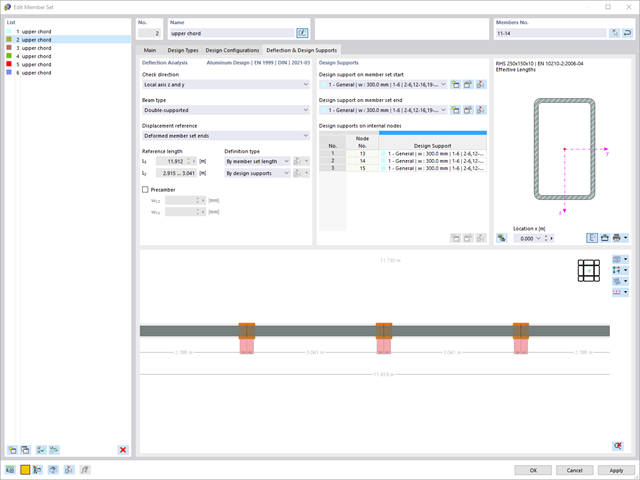
The program does a lot of work for you. For example, the load or result combinations required for the serviceability limit state are generated and calculated in RFEM/RSTAB. You can select these design situations for the deflection analysis in the Aluminum Design add-on. Depending on the specified precamber and reference system, the program determines the deformation values at each location of a member. They are then compared to the limit values.
You can specify the deformation limit value individually for each structural component in Serviceability Configuration. In this case, you define the maximum deformation depending on the reference length as the allowable limit value. By defining design supports, you can segment the components. In this way, you can determine the corresponding reference length automatically for each design direction.
And that's not all. Based on the position of the assigned design supports, the program allows you to automatically determine the distinction between beams and cantilevers. The limit value is thus determined accordingly.

Enter and model a soil solid directly in RFEM. You can combine the soil material models with all common RFEM add-ons.
This allows you to easily analyze the entire models with a complete representation of the soil-structure interaction.
All parameters required for the calculation are automatically determined from the material data that you have entered. The program then generates the stress-strain curves for each FE element.

Did you know? You can enter the soil layers that you have obtained from the subsoil expertises done in the locations into the program in the form of soil samples. Assign the explored soil materials, including their material properties, to the layers.
For the definition of the samples, you can enter the data in tables as well as in the respective editing dialog box. Furthermore, you can also specify the groundwater level in the soil samples.

The soil solids that you want to analyze are summarized in soil massifs.
Use the soil samples as a basis for a definition of the respective soil massif. This way, the program allows for user-friendly generation of the massif, including the automatic determination of the layer interfaces from the sample data, as well as the groundwater level and the boundary surface supports.
Soil massifs provide you with the option to specify a target FE mesh size independently of the global setting for the rest of the structure. You can thus consider the various requirements of the building and soil in the entire model.

Do you want to model and analyze the behavior of a soil solid? To ensure this, special suitable material models have been implemented in RFEM.
You can use the modified Mohr-Coulomb model with a linear-elastic ideal-plastic model or a nonlinear elastic model with an oedometric stress-strain relation. The limit criterion, which describes the transition from the elastic area to that of the plastic flow, is defined according to Mohr-Coulomb.

You have several options available to define masses for a modal analysis. While the masses due to self-weight are considered automatically, you can consider the loads and masses directly in a load case of the modal analysis type. Do you need more options? Select whether to consider full loads as masses, load components in the global Z-direction, or only the load components in the direction of gravity.
The program offers you an additional or alternative option for importing masses: A manual definition of load combinations as of which are the masses considered in the modal analysis. Have you selected a design standard? You can then create a design situation with the Seismic Mass combination type. Thus, the program automatically calculates a mass situation for the modal analysis according to the preferred design standard. In other words: The program creates a load combination on the basis of the preset combination coefficients for the selected standard. This contains the masses used for the modal analysis.